I recently saw an article from the EIA about residential electricity prices, which got me interested in making a map of the prices for the US. In this post I’ll show how you can use R to make a choropleth map of the average price of electricity for each state.
The data is from the the EIA; specifically the electricity retail-sales data. I went to their data browser and selected the average price for the residential sector. This gave me the URL to use to request the data from their API.
Note you will need to register for a free API key from the EIA.
Tip
I find the easiest way to store an API key in your .Renviron file is with the {usethis} package. Simply call the `usethis::edit_r_environ()` function to open the .Renviron file, add your key in the form *API_KEY="xxxxx"*, and save. After you restart R, you will be able to load the key in your code using `Sys.getenv("API_KEY")`.
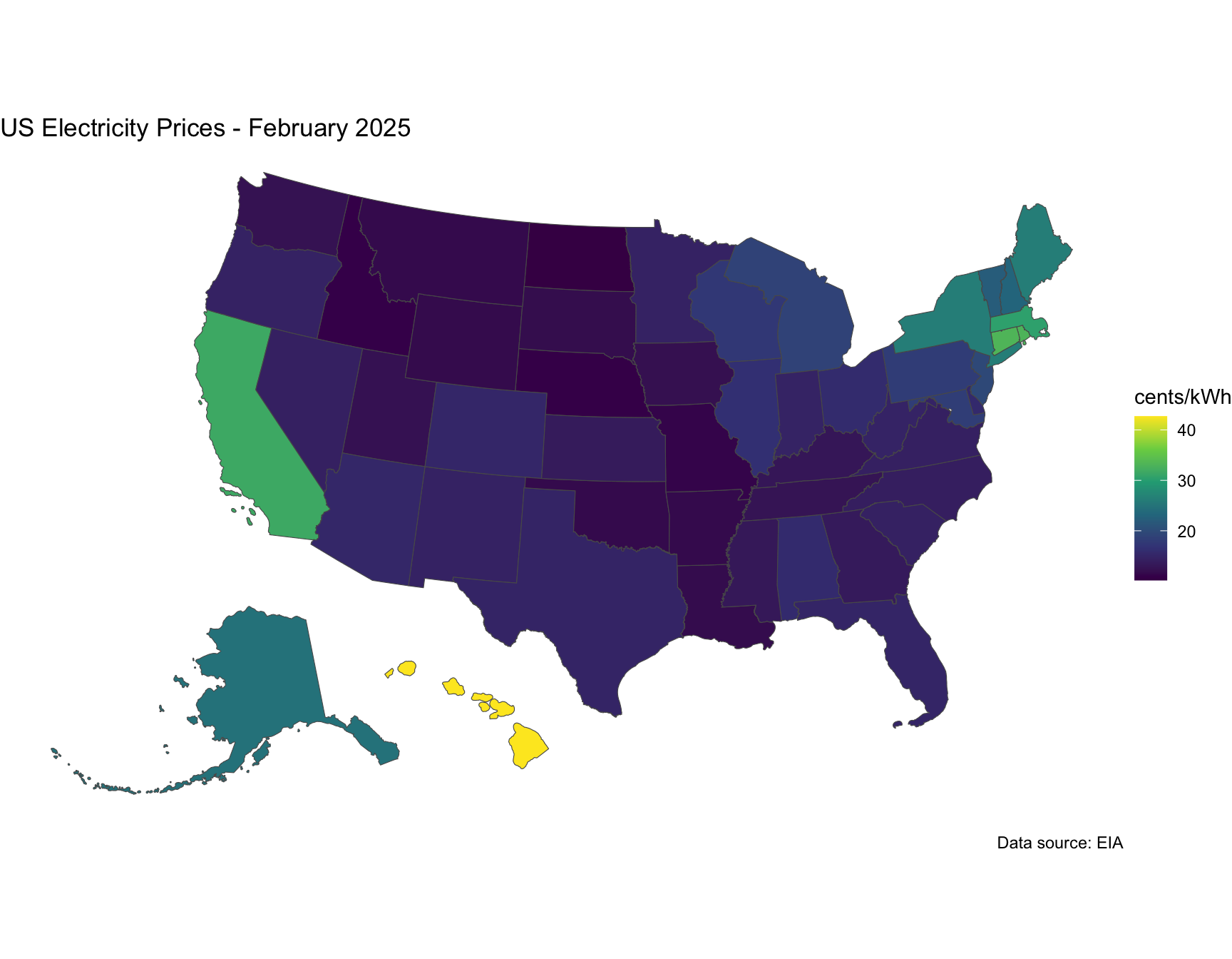
For the map, I’ll just use the prices for February 2025.
Some of the data are for regions, but I want to keep just the states. I’ll use the handy state.abb data set in R to filter the data to just US states.
Get data from API
# my API key for EIA dataapi_key <-Sys.getenv("EIA_KEY")req_url <-"https://api.eia.gov/v2/electricity/retail-sales/data/?frequency=monthly&data[0]=price&facets[sectorid][]=RES&start=2025-02&sort[0][column]=period&sort[0][direction]=desc&offset=0&length=5000"resp <- httr::GET(paste0(req_url, "&api_key=", api_key))resp_parsed <- jsonlite::fromJSON(httr::content(resp,"text"))elec_prices <- resp_parsed$response$data |>filter(period =="2025-02") |>mutate(price =as.numeric(price)) |>filter(stateid %in% state.abb)rm(resp_parsed, resp)elec_prices |> DT::datatable(options =list(pageLength =5),rownames =FALSE)
Table 1: Table of residential electricity prices for US states, from EIA.
State Geometries
Now we have the price data, but we need the states geometries to make the map. I’ll use the {tigris}(Walker 2024) package to download the states.
I also use the shift_geometry() function from {tigris} to move and re-scale Alaska and Hawaii so they fit better on the map.
Figure 1: Choropleth map of average residential electricity prices for US states. Data from EIA.
Interactive map
The static choropleth map shows the spatial variability in prices, but it would be nice to also be able to see the actual price for a state. One way to do this is to use the {ggiraph}(Gohel and Skintzos (2025)) package to add some interactivity, so that when you hover over the map the value for that state would be displayed. Unfortunately including the interactive map exceeded the size limit for my (free) blog site, but I included the code below if you are interested:
---title: "Mapping Electricity Prices with R"date: 2025-06-04image: image.pngformat: html: code-fold: show code-tools: true toc: true fig-width: 9 fig-height: 7 tbl-cap-location: bottomcode-annotations: hovereditor: visualcategories: [R,energy,API,mapping]freeze: autodraft: falsebibliography: references.bib---# IntroductionI recently saw an article from the [EIA](https://www.eia.gov/) about residential electricity prices, which got me interested in making a map of the prices for the US. In this post I'll show how you can use R to make a choropleth map of the average price of electricity for each state.```{r}#| label: libraries#| code-summary: Load Libraries#| message: falselibrary(httr) # <1>library(tidyverse) # <2>library(tigris) # <3>options(tigris_use_cache =TRUE)library(DT) # <4>library(ggiraph) # <5>```1. Get data from API2. Data Wrangling and Plotting3. Get state geometries4. Display nice data tables5. Make figures interactive# Getting the dataThe data is from the the EIA; specifically the *electricity retail-sales* data. I went to their [data browser](https://www.eia.gov/opendata/browser/electricity/retail-sales?) and selected the average price for the residential sector. This gave me the URL to use to request the data from their API.Note you will need to register for a free API key from the [EIA](https://www.eia.gov/opendata/).::: callout-tip``` I find the easiest way to store an API key in your .Renviron file is with the {usethis} package. Simply call the `usethis::edit_r_environ()` function to open the .Renviron file, add your key in the form *API_KEY="xxxxx"*, and save. After you restart R, you will be able to load the key in your code using `Sys.getenv("API_KEY")`.```:::- For the map, I'll just use the prices for February 2025.- Some of the data are for regions, but I want to keep just the states. I'll use the handy *state.abb* data set in R to filter the data to just US states.```{r}#| code-summary: Get data from API#| label: tbl-get-eia-data#| tbl-cap: "Table of residential electricity prices for US states, from EIA."#| message: false# my API key for EIA dataapi_key <-Sys.getenv("EIA_KEY")req_url <-"https://api.eia.gov/v2/electricity/retail-sales/data/?frequency=monthly&data[0]=price&facets[sectorid][]=RES&start=2025-02&sort[0][column]=period&sort[0][direction]=desc&offset=0&length=5000"resp <- httr::GET(paste0(req_url, "&api_key=", api_key))resp_parsed <- jsonlite::fromJSON(httr::content(resp,"text"))elec_prices <- resp_parsed$response$data |>filter(period =="2025-02") |>mutate(price =as.numeric(price)) |>filter(stateid %in% state.abb)rm(resp_parsed, resp)elec_prices |> DT::datatable(options =list(pageLength =5),rownames =FALSE)```# State GeometriesNow we have the price data, but we need the states geometries to make the map. I'll use the {tigris}[@tigris] package to download the states.- I also use the *shift_geometry()* function from {tigris} to move and re-scale Alaska and Hawaii so they fit better on the map.```{r}#| label: states-data#| code-summary: Get US states geometries#| message: falseus_states <- tigris::states() |>select(STUSPS, geometry) |>filter(STUSPS %in% state.abb) |> tigris::shift_geometry()head(us_states)```# Joining the dataThe last step before making the map is to join the price data with the dataframe containing the states geometries.```{r}#| label: join-data#| code-summary: Join datadat_joined <- us_states |>left_join(elec_prices, by =c("STUSPS"="stateid"))head(dat_joined,5)```# Static MapNow with the data and geometries all together, we can start making the map. First I'll make a static map (@fig-map-static) using {ggplot2}.```{r}#| label: fig-map-static#| fig-cap: Choropleth map of average residential electricity prices for US states. Data from EIA.#| code-summary: Make static mapdat_joined |>ggplot() +geom_sf(aes(fill = price)) +scale_fill_viridis_c() +theme_void() +labs(title ="US Electricity Prices - February 2025",caption ="Data source: EIA",fill ="cents/kWh") ```# Interactive mapThe static choropleth map shows the spatial variability in prices, but it would be nice to also be able to see the actual price for a state. One way to do this is to use the {ggiraph}(@ggiraph) package to add some interactivity, so that when you hover over the map the value for that state would be displayed. Unfortunately including the interactive map exceeded the size limit for my (free) blog site, but I included the code below if you are interested:```{r}#| label: fig-map-interactive#| fig-cap: Interactive choropleth map of average residential electricity prices for US states. Data from EIA.#| code-summary: Make interactive map#| eval: falseint_map <-dat_joined |>ggplot() + ggiraph::geom_sf_interactive(data = dat_joined,aes(fill = price,tooltip = price,data_id = stateDescription) ) +scale_fill_viridis_c() +theme_void() +labs(title ="US Electricity Prices - February 2025",caption ="Data source: EIA",fill ="cents/kWh") ggiraph::girafe(ggobj = int_map)```# SummaryIn this post we:-Downloaded data on electricity prices from the EIA API using {httr}[@httr]-Joined the price data with state geometries from {tigris}-Made a static choropleth map with {ggplot2}[@ggplot2]-Showed how to make the map interactive with {ggiraph}I hope you found it interesting, and maybe are inspired to adapt this analysis to make your own maps or spatial analysis!# SessionInfo::: {.callout-tip collapse="true"}## Expand for Session Info```{r, echo = FALSE}sessionInfo()```:::