Exploring US Baby Names Data

Introduction

I recently found out about a data set of popular US baby names and thought it would be interesting to analyze the data a bit in R.

Data

The data are from the US Social Security Administration. I downloaded the “National” data set from the SSA website. The data contain all baby names recorded by the SSA from 1880-2023 that applied for a social security card, except those names with fewer than 5 occurrences (to protect privacy). Some more information about the data is provided here. The data set comes as a zip file containing a folder with one csv file for each year.

library(tidyverse)# data wrangling and plotting
library(scales)   # plot axis labels
library(plotly)   # interactive plots
library(DT)       # interactive data tables

I will load a file that I already processed into a single data frame, but I wanted to explain that process here:

1. Make a list of all the csv filenames
2. Write a function to read single file into a dataframe
3. Iterate over the filenames with that function, using map() from the {purrr} Wickham and Henry (2025) package.
4. map() produces a list of dataframes. I combine them all into a single dataframe with list_rbind().

# make a list of all the filenames

data_dir <- here('data/names')

file_list <- list.files(data_dir, pattern = "*.txt")

# function to read one file
read_names_one_year <- function(file_name){
  the_df <- readr::read_csv(file.path(data_dir, file_name), col_names = c("Name", "sex", "n"))
  the_df$year <- as.integer(substr(file_name,4,7)) # get the year from the filename
  return(the_df)
}

# iterate over list of filenames; this returns a list of dataframes
dfs <- purrr::map(file_list, read_names_one_year)

# combine them all into a single dataframe
baby_names <- purrr::list_rbind(dfs)

# save the final dataframe
saveRDS(baby_names, file = here("data","baby_names_all.rds"))

# load the processed data
baby_names <- readRDS("data/baby_names_all.rds") 

glimpse(baby_names)

Rows: 2,117,219
Columns: 4
$ Name <chr> "Mary", "Anna", "Emma", "Elizabeth", "Minnie", "Margaret", "Ida",…
$ sex  <chr> "F", "F", "F", "F", "F", "F", "F", "F", "F", "F", "F", "F", "F", …
$ n    <dbl> 7065, 2604, 2003, 1939, 1746, 1578, 1472, 1414, 1320, 1288, 1258,…
$ year <int> 1880, 1880, 1880, 1880, 1880, 1880, 1880, 1880, 1880, 1880, 1880,…

Analysis

How many unique names are there in the dataset?

There are a little over 103K unique names in the data set. It seems that females have more variety in names; there are about 70K unique females names, compared to ~44K male names.

# total unique names
length(unique(baby_names$Name))

[1] 103564

# unique male names
males <- baby_names |> filter(sex == "M")
length(unique(males$Name))

[1] 44261

# unique female names
females <- baby_names |> filter(sex == "F")
length(unique(females$Name))

[1] 70903

Total births each year by sex

I wanted to check how many total male or female births were recorded each year (Figure 1). Interestingly, it looks like there tends to be more female births in the first half of the data set, and more males in the second half. This sent me down a bit of a rabbit hole. Apparently the average observed ratio of males to females is around 1.05. Interestingly, one study found that the ratio is 1 (evenly split) at conception, but increases slightly at birth. However, the data set info states “Note that many people born before 1937 never applied for a Social Security card, so their names are not included in our data” ; so I can’t tell if the ratio actually changed or is an artifact of the way data was collected.

n_year_sex <- baby_names |>
  group_by(year,sex) |>
  summarise(n_tot = sum(n))

g <- n_year_sex |>
  ggplot(aes(year, n_tot, group = sex)) +
  geom_line(aes(color = sex), linewidth = 1.3) +
  scale_y_continuous(label = comma) +
  labs(x = "Year",
       y = "Births",
       title = "Total Births Per Year")

ggplotly(g)

Figure 1: Timeseries of total births each year by sex.

Which names are the most popular over all years?

Next I looked at which baby names occur the most over all the data for both sexes (Figure 2), and separately for males (Figure 3) and females (Figure 4). There a couple male names (James, John, Robert) that are the most popular, but for females Mary is the most popular by far.

All data

baby_names |>
  group_by(Name) |>
  summarise(n_total = sum(n)) |>
  slice_max(n_total, n = 20) |>
  mutate(Name = fct_reorder(Name, n_total)) |>
  ggplot(aes(n_total, Name)) +
  geom_col(fill = "lightblue") +
  scale_x_continuous(labels = scales::label_number(scale = 1e-6, suffix = "M")) +
    labs(x = "Total Births",
       y = "",
       title = "Top 20 Names")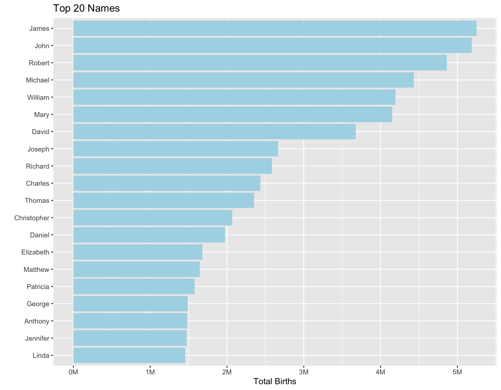

Figure 2: Top 20 most popular names over all years.

Males

baby_names |>
  filter(sex == "M") |>
  group_by(Name) |>
  summarise(n_total = sum(n)) |>
  slice_max(n_total, n = 20) |>
  mutate(Name = fct_reorder(Name, n_total)) |>
  ggplot(aes(n_total, Name)) +
  scale_x_continuous(labels = scales::label_number(scale = 1e-6, suffix = "M")) +
  geom_col(fill = "lightblue") +
    labs(x = "Total Births",
       y = "",
       title = "Top 20 Male Names")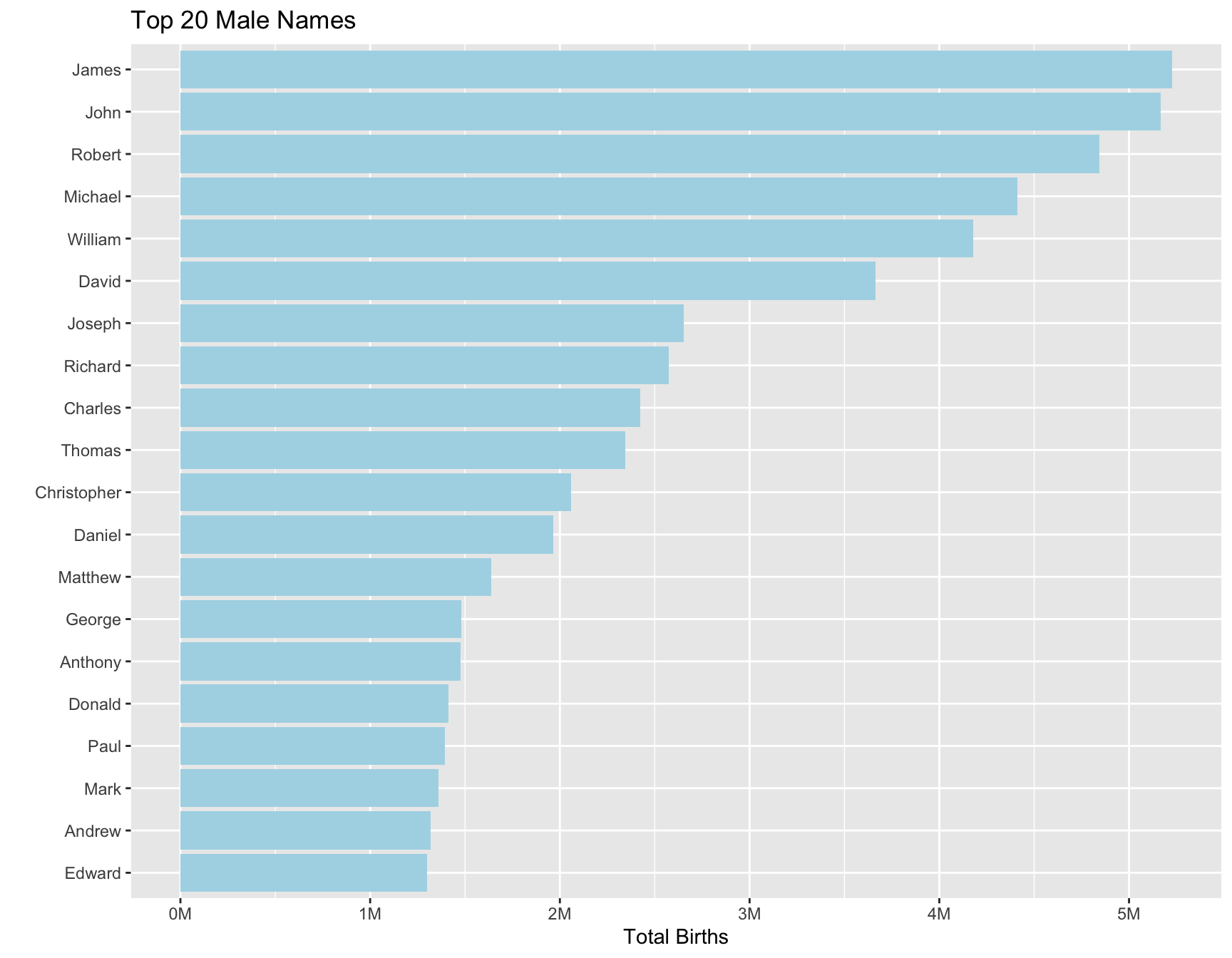

Figure 3: Top 20 most popular male names over all years.

Females

baby_names |>
  filter(sex == "F") |>
  group_by(Name) |>
  summarise(n_total = sum(n)) |>
  slice_max(n_total, n = 20) |>
  mutate(Name = fct_reorder(Name, n_total)) |>
  ggplot(aes(n_total, Name)) +
  geom_col(fill = "lightblue") +
  scale_x_continuous(labels = scales::label_number(scale = 1e-6, suffix = "M")) +
  labs(x = "Total Births",
       y = "",
       title = "Top 20 Female Names")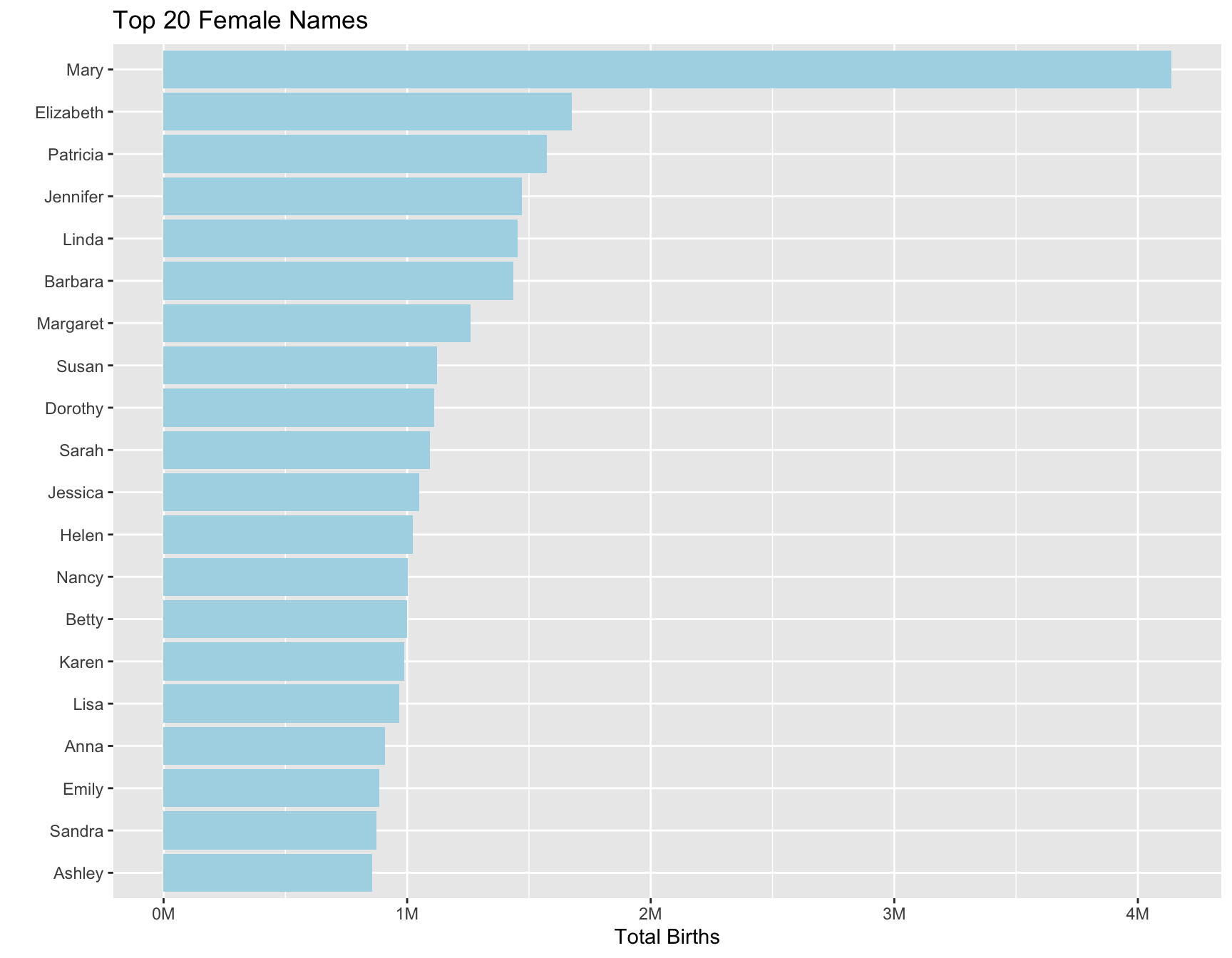

Figure 4: Top 20 most popular female names over all years.

Changes in Popularity Over Time

To see how the popularity changes over time, I plotted timeseries of the top 5 female (Figure 5) and male (Figure 6) names. There are some pretty big changes over time. Linda really had a moment around 1950, and Michael surged in popularity during the 1940’s. It’s interesting to think about what makes a name popular. I thought that some of it comes from pop culture, so I looked at the time series of Elsa. There was a dramatic spike in 2014, the year after the Frozen movie came out (though not as high as would have thought).

Females

# get the 5 most popular female names
top5_female <- baby_names |>
  filter(sex == "F") |>
  group_by(Name) |>
  summarise(n_total = sum(n)) |>
  slice_max(order_by = n_total, n = 5)


g <- baby_names |>
  filter(sex == "F") |>
  filter(Name %in% top5_female$Name) |>
  ggplot(aes(year, n, group = Name)) +
  geom_line(aes(color = Name)) +
  scale_y_continuous(label = comma) +
  labs(x = "Year",
       y = "Births",
       title = "Top 5 Female Names")

plotly::ggplotly(g)

Figure 5: Timeseries of the top 5 female names.

Males

# get the 5 most popular male names
top5_male <- baby_names |>
  filter(sex == "M") |>
  group_by(Name) |>
  summarise(n_total = sum(n)) |>
  slice_max(order_by = n_total, n = 5)


g <- baby_names |>
  filter(sex == "M") |>
  filter(Name %in% top5_male$Name) |>
  ggplot(aes(year, n, group = Name)) +
  geom_line(aes(color = Name)) +
  scale_y_continuous(label = comma) +
  labs(x = "Year",
       y = "Births",
       title = "Top 5 Male Names")

plotly::ggplotly(g)

Figure 6: Timeseries of the top 5 male names.

g <- baby_names |>
  filter(Name == "Elsa") |>
  filter(sex == "F") |>
  ggplot(aes(year,n)) +
  geom_line() +
  labs(x = "Year",
       y = "Births",
       title = "Popularity of Elsa Over Time")

ggplotly(g)

Figure 7: Births of females named “Elsa” per year.

Most popular names each year

Below is a table of the most popular male and female names each year. It looks like Liam and Olivia have dominated for the last few years (Table 1).

baby_names |>
  group_by(year, sex) |>
  slice(which.max(n)) |>
  arrange(desc(year)) |>
  select(-n) |>
  tidyr::pivot_wider(names_from = sex, values_from = Name) |>
  DT::datatable(options = list(pageLength = 10), rownames = FALSE)

Table 1: Most popular male and female names each year.

Summary

In this post I explored a dataset of US baby names, producing a number of interesting observations and questions. I hope you found it interesting, and maybe are inspired to do your own analysis!

SessionInfo

Expand for Session Info

R version 4.4.1 (2024-06-14)
Platform: x86_64-apple-darwin20
Running under: macOS 15.3.2

Matrix products: default
BLAS:   /Library/Frameworks/R.framework/Versions/4.4-x86_64/Resources/lib/libRblas.0.dylib 
LAPACK: /Library/Frameworks/R.framework/Versions/4.4-x86_64/Resources/lib/libRlapack.dylib;  LAPACK version 3.12.0

locale:
[1] en_US.UTF-8/en_US.UTF-8/en_US.UTF-8/C/en_US.UTF-8/en_US.UTF-8

time zone: America/Denver
tzcode source: internal

attached base packages:
[1] stats     graphics  grDevices datasets  utils     methods   base     

other attached packages:
 [1] DT_0.33         plotly_4.10.4   scales_1.3.0    lubridate_1.9.4
 [5] forcats_1.0.0   stringr_1.5.1   dplyr_1.1.4     purrr_1.0.4    
 [9] readr_2.1.5     tidyr_1.3.1     tibble_3.2.1    ggplot2_3.5.1  
[13] tidyverse_2.0.0

loaded via a namespace (and not attached):
 [1] sass_0.4.9        generics_0.1.3    renv_1.0.9        stringi_1.8.7    
 [5] hms_1.1.3         digest_0.6.37     magrittr_2.0.3    evaluate_1.0.3   
 [9] grid_4.4.1        timechange_0.3.0  fastmap_1.2.0     jsonlite_2.0.0   
[13] httr_1.4.7        crosstalk_1.2.1   viridisLite_0.4.2 jquerylib_0.1.4  
[17] lazyeval_0.2.2    cli_3.6.4         rlang_1.1.5       munsell_0.5.1    
[21] cachem_1.1.0      withr_3.0.2       yaml_2.3.10       tools_4.4.1      
[25] tzdb_0.5.0        colorspace_2.1-1  vctrs_0.6.5       R6_2.6.1         
[29] lifecycle_1.0.4   htmlwidgets_1.6.4 pkgconfig_2.0.3   pillar_1.10.1    
[33] bslib_0.9.0       gtable_0.3.6      glue_1.8.0        data.table_1.17.0
[37] xfun_0.51         tidyselect_1.2.1  rstudioapi_0.17.1 knitr_1.50       
[41] farver_2.1.2      htmltools_0.5.8.1 rmarkdown_2.29    labeling_0.4.3   
[45] compiler_4.4.1   

References

Wickham, Hadley, and Lionel Henry. 2025. “Purrr: Functional Programming Tools.” https://CRAN.R-project.org/package=purrr.