As you may know from a previous post I am interested in electric-vehicle (EV) trends and the transition to a more electrified transportation fleet. I wanted to do some mapping and spatial analysis, and I recently took the Creating Maps with R course by Charlie Joey Hadley, so I decided to use some of the skills I learned to create some maps of EV charging station data for Colorado.
Goal
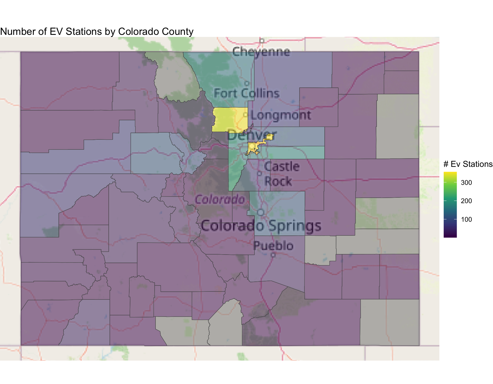
My goal in this post is to create choropleth map(s) showing the number of EV charging stations per county in Colorado.
Simple feature collection with 6 features and 12 fields
Geometry type: MULTIPOLYGON
Dimension:     XY
Bounding box:  xmin: -109.0603 ymin: 36.99891 xmax: -104.3511 ymax: 39.91418
Geodetic CRS:  NAD83
   STATEFP COUNTYFP COUNTYNS       AFFGEOID GEOID        NAME
15      08      077 00198154 0500000US08077 08077        Mesa
16      08      083 00198157 0500000US08083 08083   Montezuma
17      08      067 00198148 0500000US08067 08067    La Plata
42      08      031 00198131 0500000US08031 08031      Denver
46      08      019 00198125 0500000US08019 08019 Clear Creek
47      08      055 00198143 0500000US08055 08055    Huerfano
             NAMELSAD STUSPS STATE_NAME LSAD      ALAND   AWATER
15        Mesa County     CO   Colorado   06 8621348059 31991710
16   Montezuma County     CO   Colorado   06 5255990019 27208195
17    La Plata County     CO   Colorado   06 4376255278 25642579
42      Denver County     CO   Colorado   06  396460127  4275563
46 Clear Creek County     CO   Colorado   06 1023234059  3274900
47    Huerfano County     CO   Colorado   06 4120756290  5792101
                         geometry
15 MULTIPOLYGON (((-109.0603 3...
16 MULTIPOLYGON (((-109.0459 3...
17 MULTIPOLYGON (((-108.3796 3...
42 MULTIPOLYGON (((-104.9341 3...
46 MULTIPOLYGON (((-105.927 39...
47 MULTIPOLYGON (((-105.5013 3...
Zip codes
I have the EV station data and the county shape files, so the next step is to join them together. However, I have a problem: the EV stations data does not contain the county name or code, so I can’t join them yet without a common column. There are probably a lot of different solutions to this problem (for example the EV data contains addresses so I could geo-code these to get the county). In this case, I decided the easiest solution was to download the zip code database from the USPS (free for personal use), which contains both zip codes and their corresponding county (Table 1).
Table 2: Number of EV charging stations per county
Combining data
Now we can finally join the data we want to plot (# EV stations per county) in ev_county_counts to our sf object (co_counties) with the county spatial data, and we are ready to make some maps.
Code
co_ev_counts<-co_counties%>%left_join(ev_county_counts, by =c("NAMELSAD"="county"))co_ev_counts<-sf::st_transform(co_ev_counts, 4326)head(co_ev_counts)
Simple feature collection with 6 features and 13 fields
Geometry type: MULTIPOLYGON
Dimension:     XY
Bounding box:  xmin: -109.0603 ymin: 36.99891 xmax: -104.3511 ymax: 39.91418
Geodetic CRS:  WGS 84
  STATEFP COUNTYFP COUNTYNS       AFFGEOID GEOID        NAME           NAMELSAD
1      08      077 00198154 0500000US08077 08077        Mesa        Mesa County
2      08      083 00198157 0500000US08083 08083   Montezuma   Montezuma County
3      08      067 00198148 0500000US08067 08067    La Plata    La Plata County
4      08      031 00198131 0500000US08031 08031      Denver      Denver County
5      08      019 00198125 0500000US08019 08019 Clear Creek Clear Creek County
6      08      055 00198143 0500000US08055 08055    Huerfano    Huerfano County
  STUSPS STATE_NAME LSAD      ALAND   AWATER   n                       geometry
1     CO   Colorado   06 8621348059 31991710  61 MULTIPOLYGON (((-109.0603 3...
2     CO   Colorado   06 5255990019 27208195   5 MULTIPOLYGON (((-109.0459 3...
3     CO   Colorado   06 4376255278 25642579  39 MULTIPOLYGON (((-108.3796 3...
4     CO   Colorado   06  396460127  4275563 356 MULTIPOLYGON (((-104.9341 3...
5     CO   Colorado   06 1023234059  3274900  13 MULTIPOLYGON (((-105.927 39...
6     CO   Colorado   06 4120756290  5792101   4 MULTIPOLYGON (((-105.5013 3...
Mapping
I’m going to make choropleth maps using two of the more popular mapping packages: {ggplot2} (Wickham 2016) and {leaflet} (Cheng, Karambelkar, and Xie 2023). I think they both make good-looking maps; the main advantage to leaflet is that the map is interactive.
ggplot
{ggplot2} makes it relatively easy to plot spatial data in an sf object with the geom_sf function
Figure 1: Choropleth map of number of EV charging stations by county, made with ggplot2
Leaflet
Using {leaflet} requires a little more code but allows you to create an interactive map that can be more useful to the reader.
In the map below (Figure 2) I’ve set the popup to display the county name and number of stations when you click on the map.
You can also drag the map around and zoom in/out.
It’s also very easy with Leaflet to add a basemap (OpenStreetMap in this case) layer under the choropleth. I decided to add this here to give readers a better sense of context, and also because I wanted to highlight that the counties close to major highways (I-70 east-west and I-25 north-south) appear to have higher numbers of chargers.
Note I’ve also included some code using from the Creating Maps in R course to fix an issue in the legend where the NA entry overlaps with the other entries.
Code
# create color palettepal_ev<-leaflet::colorNumeric(palette ="viridis", domain =co_ev_counts$n)co_ev_map<-leaflet()%>%addTiles()%>%# adds OpenStretMap basemapaddPolygons(data =co_ev_counts, weight =1, color ="black", popup =paste(co_ev_counts$NAME, "<br>"," EV Stations: ", co_ev_counts$n, "<br>"), fillColor =~pal_ev(n), fillOpacity =0.6)%>%addLegend(data =co_ev_counts, pal =pal_ev, values =~n, opacity =1, title ="# of EV Stations <br> Per County")# legend fix --------------------------------------------------------------# for issue with na in legendhtml_fix<-htmltools::tags$style(type ="text/css", "div.info.legend.leaflet-control br {clear: both;}")co_ev_map%>%htmlwidgets::prependContent(html_fix)
Figure 2: Interactive choropleth map of number of EV charging stations by county. Click on a county polygon to display information.
Future Analysis
Now that I have the basic framework set up for mapping the EV data, there are a lot of other interesting questions I would like to investigate.
Look at breakdown by charger level/type/network etc..
Look at trends over time.
Look at relationship between demographics (population, income etc. ) and chargers. The tidycensus package would probably be useful for this.
Extend to other states or similar analysis at state level.
SessionInfo
In order to improve the reproducibility of this analysis, I include the sessionInfo below at the time this post was rendered.
Cheng, Joe, Bhaskar Karambelkar, and Yihui Xie. 2023. “Leaflet: Create Interactive Web Maps with the JavaScript ’Leaflet’ Library.”https://CRAN.R-project.org/package=leaflet.
---title: "Mapping the Number of EV Charging Stations by County in Colorado Using R" image: image.png format: html: code-link: true code-fold: show tbl-cap-location: bottomdate: "2023-08-01"date-modified: todaycategories: [EV, R, visualization, mapping, API]toc: truebibliography: references.bibfreeze: auto---# IntroductionAs you may know from a [previous post](https://andypicke.quarto.pub/portfolio/posts/EV_Stations/) I am interested in electric-vehicle (EV) trends and the transition to a more electrified transportation fleet. I wanted to do some mapping and spatial analysis, and I recently took the [Creating Maps with R](https://www.linkedin.com/learning-login/share?forceAccount=false&redirect=https%3A%2F%2Fwww.linkedin.com%2Flearning%2Fcreating-maps-with-r%3Ftrk%3Dshare_ent_url%26shareId%3DQgGBGCunSQyanayy1A%252Fffg%253D%253D) course by [Charlie Joey Hadley](https://www.linkedin.com/learning/instructors/charlie-joey-hadley), so I decided to use some of the skills I learned to create some maps of EV charging station data for Colorado.## Goal- My goal in this post is to create [choropleth](https://en.wikipedia.org/wiki/Choropleth_map) map(s) showing the number of EV charging stations per county in Colorado.# Data & Analysis```{r }#| label: load-libraries#| code-fold: true#| code-summary: Load LibrariessuppressPackageStartupMessages(library(tidyverse))library(httr)suppressPackageStartupMessages(library(jsonlite))ggplot2::theme_set(theme_grey(base_size = 15))library(leaflet)suppressPackageStartupMessages(library(tigris)) # to get county shapefiles for mapslibrary(ggspatial) # for adding basemaps to ggplot2 mapslibrary(DT) # make nice data tables```## EV Stations dataData on EV stations is obtained from the [Alternative Fuels Data Center](https://afdc.energy.gov/)'s Alternative Fuel Stations [database](https://developer.nrel.gov/docs/transportation/alt-fuel-stations-v1/). See my [previous post](https://andypicke.quarto.pub/portfolio/posts/EV_Stations/){.uri} for more details on getting the data from the [API](https://developer.nrel.gov/docs/transportation/alt-fuel-stations-v1/all/).```{r }#| label: load-data#| code-fold: true#| code-summary: Load EV stations data from API# API key is stored in my .Renviron fileapi_key <- Sys.getenv("AFDC_KEY")target <- "https://developer.nrel.gov/api/alt-fuel-stations/v1"# Return data for all electric stations in Coloradoapi_path <- ".json?&fuel_type=ELEC&state=CO&limit=all"complete_api_path <- paste0(target,api_path,'&api_key=',api_key)response <- httr::GET(url = complete_api_path)if (response$status_code != 200) { print(paste('Warning, API call returned error code', response$status_code))}ev_dat <- jsonlite::fromJSON(httr::content(response,"text"))ev <- ev_dat$fuel_stations# filter out non-EV related fieldsev <- ev %>% select(-dplyr::starts_with("lng")) %>% select(-starts_with("cng")) %>% select(-starts_with("lpg")) %>% select(-starts_with("hy")) %>% select(-starts_with("ng")) %>% select(-starts_with("e85")) %>% select(-starts_with("bd")) %>% select(-starts_with("rd")) %>% filter(status_code == 'E')```## County dataNext I need shape files for the Colorado counties to make the map; these are obtained from the [{tigris}](https://github.com/walkerke/tigris)[@tigris] package.```{r }#| label: get-county-dataoptions(tigris_use_cache = TRUE)co_counties <- tigris::counties("CO",cb = TRUE, progress_bar = FALSE)head(co_counties)```## Zip codesI have the EV station data and the county shape files, so the next step is to join them together. However, I have a **problem**: the EV stations data does not contain the county name or code, so I can't join them yet without a common column. There are probably a lot of different solutions to this problem (for example the EV data contains addresses so I could geo-code these to get the county). In this case, I decided the easiest solution was to download the [zip code database](https://www.unitedstateszipcodes.org/zip-code-database/){.uri} from the USPS (free for personal use), which contains both zip codes and their corresponding county (@tbl-zip-codes).```{r }#| label: tbl-zip-codes#| tbl-cap: Zip code data from USPSzips <- readr::read_csv("data/zip_code_database.csv", show_col_types = FALSE) %>% filter(state == "CO") %>% select(zip, primary_city, county)zips |> DT::datatable(options = list(pageLength = 5), rownames = FALSE)```Next I compute the number of stations per zip code in the EV data, and join to the zip code database to add the county column (@tbl-ev-county-counts).```{r }#| label: tbl-ev-county-counts#| tbl-cap: Number of EV charging stations per countyev_county_counts <- ev %>% select(id,zip,city) %>% left_join(zips, by = "zip") %>% dplyr::count(county) %>% arrange(desc(n))ev_county_counts |> DT::datatable(options = list(pageLength = 5), rownames = FALSE)```## Combining dataNow we can finally join the data we want to plot (# EV stations per county) in *ev_county_counts* to our sf object (*co_counties*) with the county spatial data, and we are ready to make some maps.```{r Combine Data}co_ev_counts <- co_counties %>% left_join(ev_county_counts, by = c("NAMELSAD" = "county"))co_ev_counts <- sf::st_transform(co_ev_counts, 4326)head(co_ev_counts)```# MappingI'm going to make choropleth maps using two of the more popular mapping packages: {*ggplot2*} [@ggplot2] and {*leaflet*} [@leaflet]. I think they both make good-looking maps; the main advantage to leaflet is that the map is interactive.## ggplot- {ggplot2} makes it relatively easy to plot spatial data in an sf object with the *geom_sf* function- The {*scales*} [@scales] package is used to format the numbers in the legend- The {*ggspatial*} [@ggspatial] package is used to add a base map showing some of the major cities and roads```{r }#| label: fig-ggplot-choropleth#| fig-cap: Choropleth map of number of EV charging stations by county, made with ggplot2ggplot() + ggspatial::annotation_map_tile(progress = "none") + geom_sf(data = co_ev_counts, aes(fill = n), alpha = 0.5) + scale_fill_viridis_c(labels = scales::number_format(big.mark = ","), name = '# Ev Stations') + ggtitle("Number of EV Stations by Colorado County") + theme_void()```## LeafletUsing {leaflet} requires a little more code but allows you to create an interactive map that can be more useful to the reader.\- In the map below (@fig-leaflet-choropleth) I've set the *popup* to display the county name and number of stations when you **click on the map**.- You can also **drag the map around and zoom in/out**.- It's also very easy with Leaflet to add a basemap (OpenStreetMap in this case) layer under the choropleth. I decided to add this here to give readers a better sense of context, and also because I wanted to highlight that the counties close to major highways (I-70 east-west and I-25 north-south) appear to have higher numbers of chargers.- Note I've also included some code using from the [Creating Maps in R](https://www.linkedin.com/learning-login/share?forceAccount=false&redirect=https%3A%2F%2Fwww.linkedin.com%2Flearning%2Fcreating-maps-with-r%3Ftrk%3Dshare_ent_url%26shareId%3DQgGBGCunSQyanayy1A%252Fffg%253D%253D) course to fix an issue in the legend where the NA entry overlaps with the other entries.```{r }#| label: fig-leaflet-choropleth#| fig-cap: Interactive choropleth map of number of EV charging stations by county. Click on a county polygon to display information.# create color palettepal_ev <- leaflet::colorNumeric(palette = "viridis", domain = co_ev_counts$n)co_ev_map <- leaflet() %>% addTiles() %>% # adds OpenStretMap basemap addPolygons(data = co_ev_counts, weight = 1, color = "black", popup = paste(co_ev_counts$NAME, "<br>", " EV Stations: ", co_ev_counts$n, "<br>"), fillColor = ~pal_ev(n), fillOpacity = 0.6) %>% addLegend(data = co_ev_counts, pal = pal_ev, values = ~n, opacity = 1, title = "# of EV Stations <br> Per County" )# legend fix --------------------------------------------------------------# for issue with na in legendhtml_fix <- htmltools::tags$style(type = "text/css", "div.info.legend.leaflet-control br {clear: both;}") co_ev_map %>% htmlwidgets::prependContent(html_fix)```# Future AnalysisNow that I have the basic framework set up for mapping the EV data, there are a lot of other interesting questions I would like to investigate.- Look at breakdown by charger level/type/network etc..- Look at trends over time.- Look at relationship between demographics (population, income etc. ) and chargers. The [*tidycensus*](https://walker-data.com/tidycensus/) package would probably be useful for this.- Extend to other states or similar analysis at state level.# SessionInfoIn order to improve the reproducibility of this analysis, I include the *sessionInfo* below at the time this post was rendered.# SessionInfo::: {.callout-tip collapse="true"}## Expand for Session Info```{r, echo = FALSE}sessionInfo()```:::# References