Analyzing Trends in Heating and Cooling Degree days using R

Introduction

Degree days are useful as a measure of building heating and cooling demands. A degree day is calculated as the difference between the average temperature (the average of the high and low temperature for the day) and a reference temperature (in the US 65°F is used). For example, if the average temperature today is 40°F, that would be 25 heating degree days (HDD). A summer day with an average temperature of 85°F would have 20 cooling degree days (CDD). Degree days are usually well correlated with the amount of energy used to heat or cool a home.

I was interested in obtaining and analyzing degree day data; in particular I wanted to see if there were any noticeable trends over time. Given an overall increase in earth’s average temperature due to climate change, I would hypothesize that there might be an overall increase in CDD and a decrease in HDD.

Changes in heating or cooling degree days would have implications for the amount of energy needed in the future to heat and cool residential or commercial buildings, resulting changes in demand on the electric grid, and implications for related carbon emissions (either for the power grid or from burning fossil fuels to heat buildings).

Data

I obtained heating and cooling degree day data from the U.S. Energy Information Administration for the US. Note these data are weighted by population, to reflect the effect of both temperature and population on energy demands for cooling and heating. You can see details of how the EIA data are calculated here.

suppressPackageStartupMessages(library(tidyverse))
ggplot2::theme_set(theme_grey(base_size = 15))
suppressPackageStartupMessages(library(janitor))
library(broom)
suppressPackageStartupMessages(library(DT))
suppressPackageStartupMessages(library(plotly))

I’ll only use years we have complete data for (1997-2022). Table 1 shows the data after being loaded and cleaned up.

region <- "u_s"

dd <- read_csv(paste0('data/EIA_DegreeDays_Monthly_',region,'.csv'), 
               skip = 4,
               show_col_types = FALSE) |>
  janitor::clean_names() |>
  rename(CDD = paste0('cooling_degree_days_',region,
                      '_cooling_degree_days_cooling_degree_days')) |>
  rename(HDD = paste0('heating_degree_days_',region,
                      '_heating_degree_days_heating_degree_days')) |>
  mutate(date = lubridate::my(month)) |>
  select(-month) |>
  mutate(month = lubridate::month(date)) |>
  mutate(year = lubridate::year(date)) |>
  filter(year > 1996, year < 2023) # keep only complete years

dd |>
  DT::datatable(options = list(pageLength = 5), rownames = FALSE)

Table 1: Table of monthly degree day data for US

I’ll also make a dataframe of the yearly totals (Table 2)

dd_yearly <- dd |>
  filter(year > 1996) |>
  group_by(year) |>
  summarise(HDD = sum(HDD, na.rm = TRUE),
            CDD = sum(CDD, na.rm = TRUE)
            )

dd |>
  DT::datatable(options = list(pageLength = 5), rownames = FALSE)

Table 2: Table of yearly degree days for the US

Analysis

Heating Degree Days

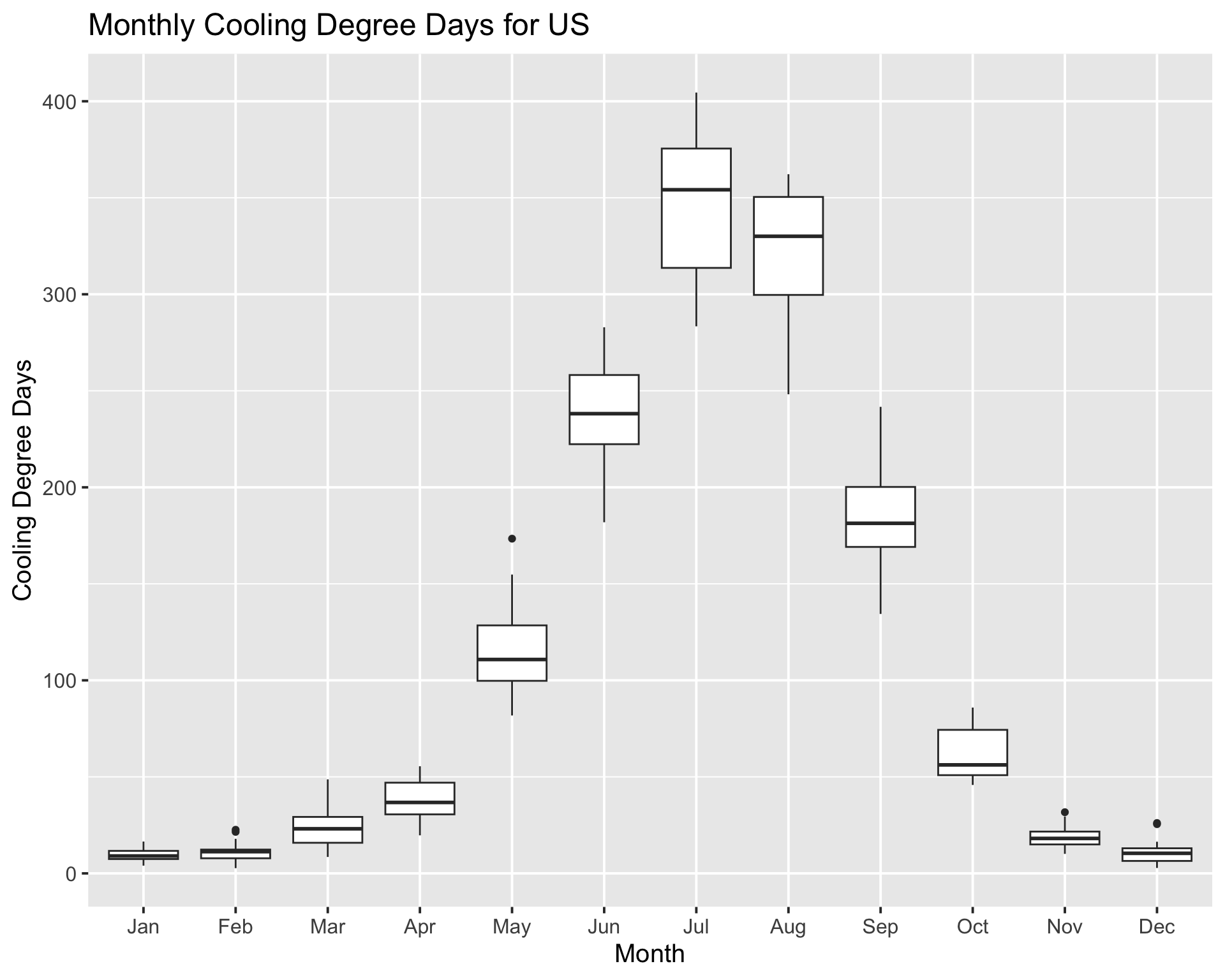
Figure 1 shows the distribution (using a boxplot) of US heating degree days for each month. Not surprisingly HDD tends to be higher in winter months, although there is a decent amount of variability between years.

HDD Per Month

dd |>
  mutate(month_name = lubridate::month(date, label = TRUE)) |>
  ggplot(aes(month_name, HDD, group = month_name)) +
  geom_boxplot() +
  labs(title = 'Monthly Heating Degree Days for US (1997-2022)',
       x = 'Month',
       y = "Heating Degree Days")

Figure 1: Boxplot of US heating degree days for each month

Trends in HDD

Is there a trend in HDD over time? I would expect that HDD might decrease over time due to climate change and the increase in earth’s average temperature.

Annual

Figure 2 shows a timeseries of the annual total heating degree days in the US, along with a linear regression line that shows a negative trend.

g <- dd_yearly |>
  ggplot(aes(year, HDD)) +
  geom_point(size = 4, alpha = 0.5) +
  geom_smooth(method = 'lm', formula = 'y~x') +
  labs(title = "US Annual Heating Degree Days")


plotly::ggplotly(g)

Figure 2: Timeseries of annual US HDD

hdd_yearly_fit <- lm(data = dd_yearly, formula = 'HDD ~ year')

broom::tidy(hdd_yearly_fit) |> mutate_if(is.numeric,~round(.x,digits = 3)) |>
  DT::datatable()

Table 3: Results of linear regression for annual HDD

There is a fair bit of variability, but looking at the fit metrics (Table 3) shows that the negative trend in HDD is statistically significant (p-value < 0.05). Annual heating degree days are decreasing at a rate of 13 HDD per year.

Monthly

We have seen that there is a negative trend in annual HDD; what are the trends for individual months? Figure 3 shows timeseries of monthly HDD vs year for winter months, with linear regression lines plotted over them. Visually there appears to be a negative trend for some of the months.

dd |>
  filter(month %in% c(11,12,1,2,3,4)) |>
  mutate(month_name = lubridate::month(date, label = TRUE)) |>
  ggplot(aes(year, HDD, group = month_name)) +
  geom_point(size = 3, alpha = 0.5) +
  geom_smooth(method = 'lm', formula = 'y ~ x') +
  facet_wrap('month_name', scales = 'free') +
  guides(x =  guide_axis(angle = 45))

Figure 3: HDD vs year for winter months

To better quantify these trends I want to fit a linear regression to the data for each month and examine the results. This could be done with a for loop, but I will take advantage of a nice nested workflow using the tidyr (Wickham, Vaughan, and Girlich 2023), broom (Robinson, Hayes, and Couch 2023), and purrr (Wickham and Henry 2023) packages.

dd_fit_hdd <- dd |>
  group_by(month) |>
  nest() |>
  mutate(fit = map(data, ~ lm(HDD ~ year, data = .x) ),
         tidied = map(fit, broom::tidy),
         glanced = map(fit, broom::glance)
  ) %>%
  unnest(tidied) |>
  ungroup()

dd_fit_hdd |>
  mutate_if(is.numeric,~round(.x,digits = 3)) |>
  DT::datatable(rownames = FALSE, options = list(pageLength = 5))

Table 4: Results of linear regression fits of heating degree days for each month

Now that the data and model fit results are in a tidy dataframe (Table 4), they can be easily filtered to identify significant fits using p-values (Table 5). The months with significant trends are June, August, September, and October. These months and the linear regression lines are shown in Figure 4

dd_fit_hdd  |>
  filter(term == 'year') |>
  filter(p.value < 0.05) |>
  mutate_if(is.numeric,~round(.x,digits = 3)) |>
  select(-c(data, fit, term, glanced)) |>
  DT::datatable(rownames = FALSE)

Table 5: Table of significant HDD fits (based on p-value < 0.05)

dd |>
  filter(month %in% c(6,8,9,10)) |>
  mutate(month_name = lubridate::month(date, label = TRUE)) |>
  ggplot(aes(year, HDD, group = month_name)) +
  geom_point(size = 4, alpha = 0.5) +
  geom_smooth(method = 'lm', formula = 'y ~ x') +
  facet_wrap('month_name', scales = 'free')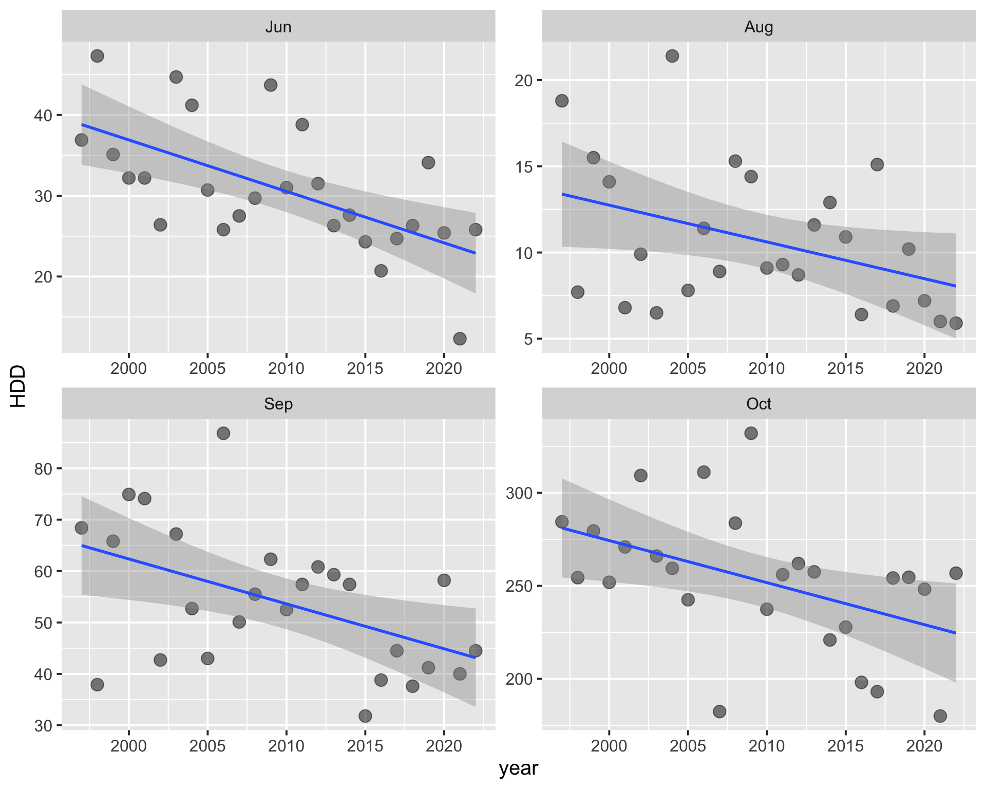 

Figure 4: HDD vs year for months with signficant trends

Cooling Degree Days

CDD Per Month

Figure 5 shows the distribution of US heating degree days for each month. Not surprisingly CDD tends to be higher in summer months, although there is a decent amount of variability between years.

dd |>
  mutate(month_name = lubridate::month(date, label = TRUE)) |>
  ggplot(aes(month_name, CDD, group = month_name)) +
  geom_boxplot() +
  labs(title = 'Monthly Cooling Degree Days for US',
       x = 'Month',
       y = "Cooling Degree Days")

Figure 5: Boxplot of US cooling degree days for each month

Trends in CDD

Annual

Is there a trend in CDD over time? I would expect that CDD might increase over time due to climate change and the increase in earth’s average temperature.

Figure 6 shows a timeseries of the annual total heating degree days in the US, along with a linear regression line showing a positive trend.

g <- dd_yearly |>
  ggplot(aes(year, CDD)) +
  geom_point(size = 4, alpha = 0.5) +
  geom_smooth(method = 'lm', formula = 'y~x') +
  labs(title = "US Annual Cooling Degree Days")

plotly::ggplotly(g)

Figure 6: Timeseries of annual US CDD

cdd_yearly_fit <- lm(data = dd_yearly, formula = 'CDD ~ year')

broom::tidy(cdd_yearly_fit) |> 
  mutate_if(is.numeric,~round(.x,digits = 3)) |>
  DT::datatable()

Table 6: Results of linear regression for annual CDD

Looking at the fit metrics shows that the positive trend in CDD is indeed statistically significant (Table 6), with CDD increasing at a rate of 12.28

Monthly

Figure 7 shows timeseries of monthly CDD vs year for the 4 summer months with the highest CDD, with linear regression lines plotted over them. Visually there appears to be a positive trend for each month.

dd |>
  filter(month %in% c(6,7,8,9)) |>
  mutate(month_name = lubridate::month(date, label = TRUE)) |>
  ggplot(aes(year, CDD, group = month_name)) +
  geom_point(size = 4, alpha = 0.5) +
  geom_smooth(method = 'lm', formula = 'y ~ x') +
  facet_wrap('month_name')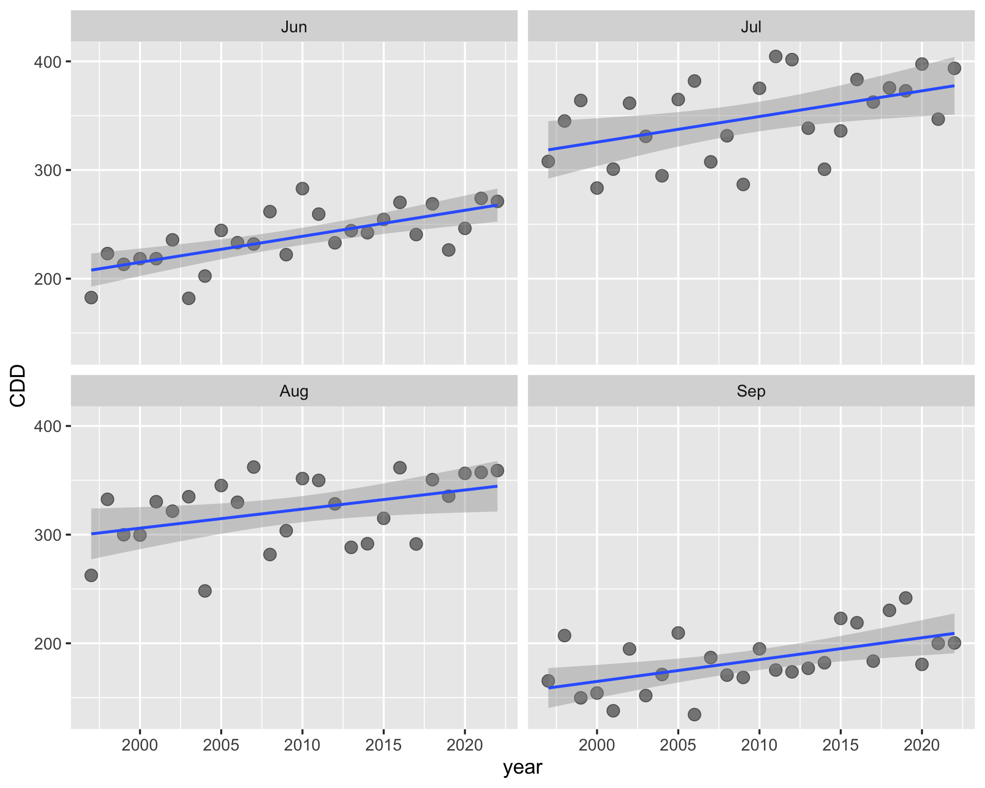

Figure 7: CDD vs year for summer month

Next I’ll apply a linear regression to each month using the same workflow used for HDD.

dd_fit_cdd <- dd |>
  group_by(month) |>
  nest() |>
  mutate(fit = map(data, ~ lm(CDD ~ year, data = .x) ),
         tidied = map(fit, broom::tidy)
  ) %>%
  unnest(tidied) |>
  ungroup()

There are significant positive trends in CDD for July, August, September, October, and December (Table 7). Figure 8 shows the data and fits for these months in detail.

dd_fit_cdd  |>
  filter(term == 'year') |>
  filter(p.value < 0.05) |>
  mutate_if(is.numeric,~round(.x,digits = 3)) |>
  select(-c(data, fit, term)) |>
  DT::datatable(rownames = FALSE,options = list(pageLength = 5))

Table 7: Table of significant CDD fits

dd |>
  filter(month %in% c(7,8,9,10,12)) |>
  mutate(month_name = lubridate::month(date, label = TRUE)) |>
  ggplot(aes(year, CDD, group = month_name)) +
  geom_point(size = 4, alpha = 0.5) +
  geom_smooth(method = 'lm', formula = 'y ~ x') +
  facet_wrap('month_name', scales = 'free') +
  guides(x =  guide_axis(angle = 45))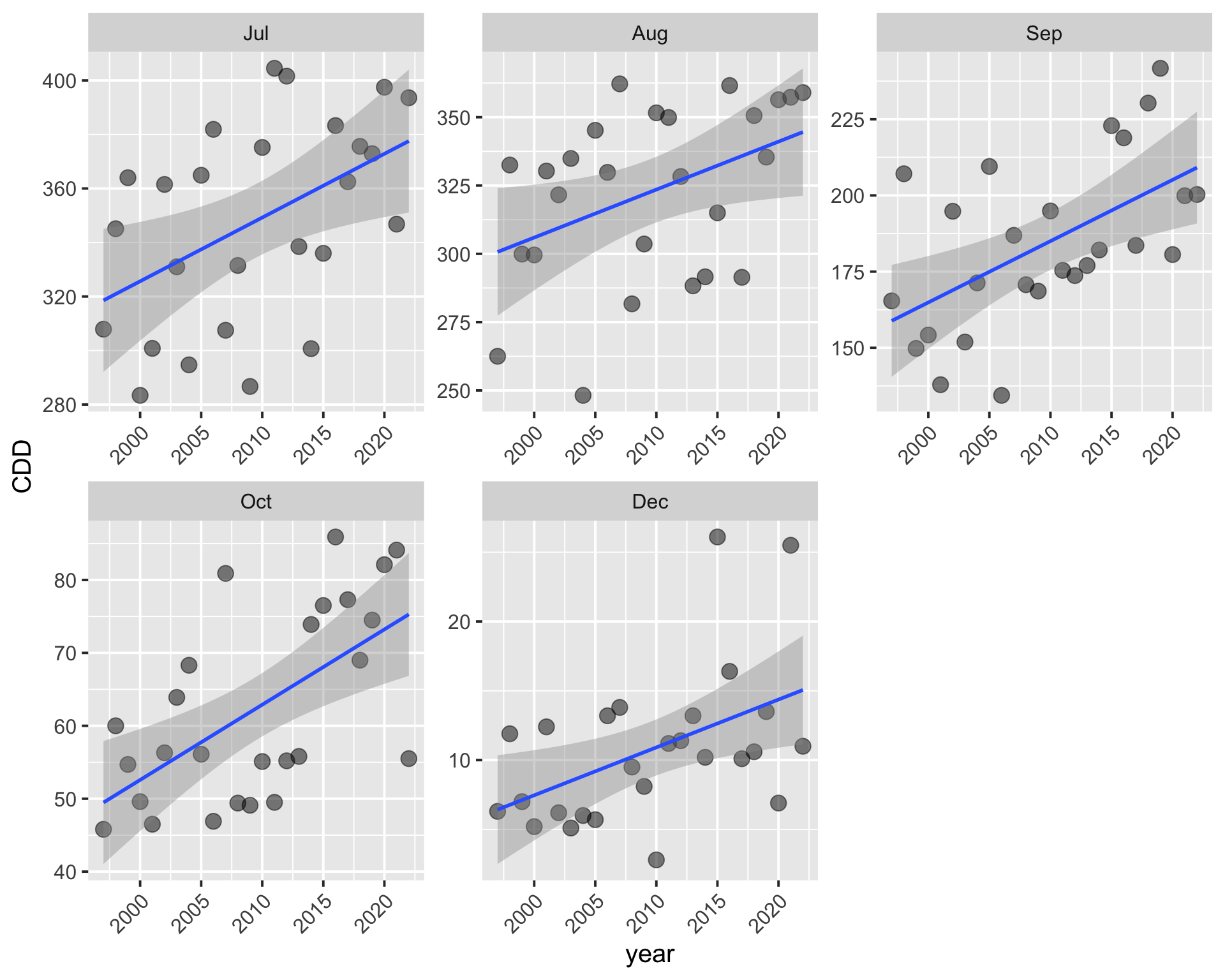

Figure 8: CDD vs year for Months with significant trends

Summary

Annual and monthly heating and cooling degree days for the US 1997-2022 were analyzed. A linear regression was applied to the annual data, and to each month, to determine if there was a trend. Model fits with a p-value less than 0.05 were considered significant.

• There is a negative trend in annual HDD (Figure 2, Table 3), with HDD decreasing at a rate of 13.2 HDD per year.

• There is a positive trend in annual CDD (Figure 6, Table 6), with CDD increasing at a rate of 12.28 CDD per year.

• There are significant negative trends in HDD for the months of June, August, September, and October (Table 5).

• There are significant positive trends in CDD for the months of July, August, September, October, and December (Table 7).

Future Research Questions

Implications for energy use

• How much actual energy use (kWh, therms, etc.) corresponds to a degree day? This will depend on many factors, but we could make a rough estimate by comparing degree days to energy demand or consumption.

SessionInfo

To enhance reproducibility, my sessionInfo is included below:

sessionInfo()

R version 4.3.1 (2023-06-16)
Platform: x86_64-apple-darwin20 (64-bit)
Running under: macOS Sonoma 14.2

Matrix products: default
BLAS:   /Library/Frameworks/R.framework/Versions/4.3-x86_64/Resources/lib/libRblas.0.dylib 
LAPACK: /Library/Frameworks/R.framework/Versions/4.3-x86_64/Resources/lib/libRlapack.dylib;  LAPACK version 3.11.0

locale:
[1] en_US.UTF-8/en_US.UTF-8/en_US.UTF-8/C/en_US.UTF-8/en_US.UTF-8

time zone: America/Denver
tzcode source: internal

attached base packages:
[1] stats     graphics  grDevices datasets  utils     methods   base     

other attached packages:
 [1] plotly_4.10.3   DT_0.30         broom_1.0.5     janitor_2.2.0  
 [5] lubridate_1.9.3 forcats_1.0.0   stringr_1.5.0   dplyr_1.1.3    
 [9] purrr_1.0.2     readr_2.1.4     tidyr_1.3.0     tibble_3.2.1   
[13] ggplot2_3.4.4   tidyverse_2.0.0

loaded via a namespace (and not attached):
 [1] gtable_0.3.4      xfun_0.40         bslib_0.5.1       htmlwidgets_1.6.2
 [5] lattice_0.22-5    tzdb_0.4.0        vctrs_0.6.4       tools_4.3.1      
 [9] crosstalk_1.2.0   generics_0.1.3    parallel_4.3.1    fansi_1.0.5      
[13] pkgconfig_2.0.3   Matrix_1.6-1.1    data.table_1.14.8 lifecycle_1.0.3  
[17] farver_2.1.1      compiler_4.3.1    munsell_0.5.0     snakecase_0.11.1 
[21] htmltools_0.5.6.1 sass_0.4.7        yaml_2.3.7        lazyeval_0.2.2   
[25] pillar_1.9.0      crayon_1.5.2      jquerylib_0.1.4   ellipsis_0.3.2   
[29] cachem_1.0.8      nlme_3.1-163      tidyselect_1.2.0  digest_0.6.33    
[33] stringi_1.7.12    splines_4.3.1     labeling_0.4.3    fastmap_1.1.1    
[37] grid_4.3.1        colorspace_2.1-0  cli_3.6.1         magrittr_2.0.3   
[41] utf8_1.2.4        withr_2.5.1       scales_1.2.1      backports_1.4.1  
[45] bit64_4.0.5       timechange_0.2.0  rmarkdown_2.25    httr_1.4.7       
[49] bit_4.0.5         hms_1.1.3         evaluate_0.22     knitr_1.44       
[53] viridisLite_0.4.2 mgcv_1.9-0        rlang_1.1.1       glue_1.6.2       
[57] renv_1.0.3        rstudioapi_0.15.0 vroom_1.6.4       jsonlite_1.8.7   
[61] R6_2.5.1         

References

Robinson, David, Alex Hayes, and Simon Couch. 2023. “Broom: Convert Statistical Objects into Tidy Tibbles.” https://CRAN.R-project.org/package=broom.

Wickham, Hadley, and Lionel Henry. 2023. “Purrr: Functional Programming Tools.” https://CRAN.R-project.org/package=purrr.

Wickham, Hadley, Davis Vaughan, and Maximilian Girlich. 2023. “Tidyr: Tidy Messy Data.” https://CRAN.R-project.org/package=tidyr.